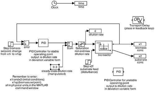
M7.5 SIMULINK Model File

In order to save time on constructing your block diagram, copy the block for the bioreactor from the textbook web page (see Figure M7-2)

biofbc.mdl

I recommend that you make your proportional and integral terms in the PID controller a function of lambda (l). Then, before each simulation run, you merely have to type in a new lambda in the MATLAB window, rather than typing in new PI parameters. Always realize that the integral term in the default SIMULINK PID block is our k_c/t_I.

Notice that the SIMULINK diagram contains two extra blocks. The transport delay block can be inserted in the feedback loop to illustrate the effects of a measurement time delay. The PID controller for the open-loop unstable point can be inserted when Additional Exercise 2 is being solved.

The following must be entered into the MATLAB command window: initial conditions, x1i and x2i; setpoint for biomass concentration, x1sp; final simulation time, tfinal; substrate feed concentration, x2f; and the IMC filter factor, lambda.

• The transfer function parameters are used by the PID controller block. The IMC-based PID parameters are different depending on whether the process is open-loop stable (Additional Exercise 1) or open-loop unstable (Additional Exercise 2). This is also seen by comparing Tables 9-1 and 9-3.

• Notice that a saturation block is used so that the dilution rate is bounded between 0.0 and 0.6. This is consistent with "real-world" constraints on manipulated variable action.

• The typical rule-of-thumb for l for open-loop stable systems is roughly one third to one half of the dominant time constant. There are no good rules-of-thumb for open-loop unstable systems.

When performing your simulations, plot the dilution rate to see if it is hitting a constraint.