M7.4 Unstable Steady-State Operating Point

Design an IMC-based PID controller to control the bioreactor at equilibrium point 2—the unstable nontrivial point. The steady state (also use this as the initial condition for your simulations) is

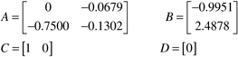
At this point, the state space model is

graphics/m07equ11.gif

Use MATLAB to find that the eigenvalues are –0.3 and 0.169836 hr^-1, so the system is unstable and the IMC-based PID method for unstable systems must be used (Table 9-3). Find the transfer function relating the dilution rate to the biomass concentration and use this for controller design. You may wish to use the MATLAB function ss2tf to find the process transfer function

After placing the process model in gain and time constant form (and cancelling common poles and zeros), you should find

That is, the transfer function has a RHP pole at 0.1698 hr^-1 which is consistent with the state space model. Notice that we can use the first entry in Table 9-3, which is a PI controller.

Show how the response to a small setpoint change varies with l (show explicitly how the PID tuning parameters vary with l). I suggest setpoint changes from 0.995103 to 0.985 and 1.005 g/liter.
For a particular value of l, show how the magnitude of the setpoint change affects your response. This is where the nonlinearity comes into play. Try changing from the steady-state value of 0.995013 to 0.5, 0.75, 1.5, and 2.0 g/liter.
Use the transport delay block in SIMULINK. Start with q = 0.25 hour and discuss how the time delay affects your choice of l.
Consider now disturbance rejection. Do not make a setpoint change but do make a step change in substract feed concentration (x_2f) from 4 to 3.5 gmol/liter at t = 1 hour.

[ Team LiB ]