13.8 Using the RGA to Determine Variable Pairings

In the previous section, we showed how to tune controllers, assuming that a decision on the pairing had already been established. The purpose of this section is to give some examples to illustrate how inputs and outputs should be paired to form MVSISO control loops.

Example 13.1, continued

Consider the whiskey-blending problem, which had the steady-state process gain matrix and RGA:

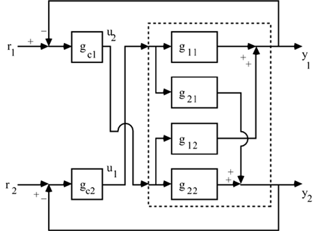
indicating that the output-input pairings should be y₁-u₂ and y₂-u₁. In order to achieve this pairing, we could use the block diagram shown in Figure 13-13.

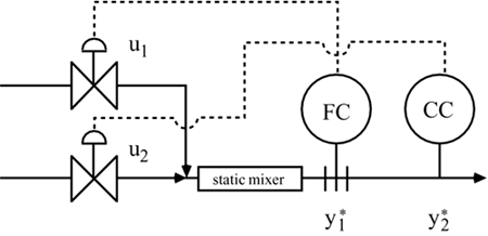
Notice that the difference between r₂ and y₂ (the error in output 2) is used to adjust u₁, using a PID controller (g_c1), hence, we refer to this pairing as y₂-u₁. Similarly, the difference between r₁ and y₁ (the error in output 1) is used to adjust u₂, using a PID controller (g_c1); hence, we refer to this pairing as y₁-u₂. This corresponds to the physical diagram shown in Figure 13-3b.

An alternative is to rearrange (renumber) our outputs or inputs so that the natural pairing is y₁-u₁ and y₂-u₂ (in the renumbered variables). For example, we could renumber the outputs. Let and , where * indicates the newly redefined variable. This corresponds to the control and instrumentation diagram shown in Figure 13-14.

We can write

or

The reader should verify that the new RGA is

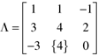
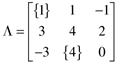
Notice that redefining the outputs is equivalent to switching the rows of the process gain matrix related to the corresponding outputs (in this case, switching rows 1 and 2 is equivalent to exchanging outputs 1 and 2). The new RGA is found by making the same transformation of rows in the RGA, as was performed on the process gain matrix.

Similarly, redefining the inputs is equivalent to switching the columns of the process gain matrix related to the corresponding inputs. The new RGA is found by making the same transformation of columns in the RGA, as was performed on the process gain matrix.

Generalization

We have shown, by way of example, that outputs can be renumbered by switching the rows in the process gain matrix, and inputs can be renumbered by switching columns in the process gain matrix. Each time we perform this exchange of variables, we do not need to recalculate the relative gain array—we simply find the new RGA by performing the same row and column exchanges on the RGA that we performed on the process gain matrix. By performing this exchange (renumbering) of variables, we can always rearrange our inputs and outputs such that loop 1 has a pairing of y₁ and u₁ (in the newly defined variables). For this reason, we will often assume that a y₁-u₁ pairing has been made and discuss the effect of l₁₁ on controller tuning.

Example 13.4: A Three Input–Three Output System

Consider the following RGA for a system with three inputs and three outputs:

How would you choose input-output pairings for this process?

Solution:

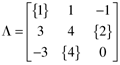
Look at row 3 in the relative gain array; this corresponds to output 3. We would not pair y₃ with u₃ because of the 0 term. We also would not pair y₃ with u₁ because of the –3 term. This means that y₃ must be paired with u₂. Let us indicate this choice in our RGA,

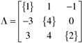
Now we have eliminated the third output (row) and the second input (column) from our selection process. From the first row (output), we see that we would not pair y₁ with u₃ because of the –1 term. We also cannot pair y₁ with u₂ because we have already paired u₂ with y₃ (hence, the circle). Our only choice is to pair y₁ with u₁. Let us indicate this choice in our RGA,

Now, we have eliminated outputs 1 and 3 (rows 1 and 3) as well as inputs 1 and 2 (columns 1 and 2). We have no choice but to pair y₂ with u₃, and we make that choice below:

Notice also, that we can renumber our outputs, such that pairings of the new variables occur on the diagonal. For example, if we define and , this is equivalent to switching the second and third rows to obtain

which is based on the new output vector

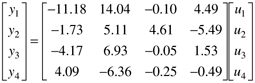
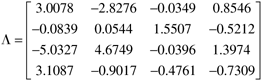
Example 13.5: A Four Input–Four Output Distillation Column (Alatiqi and Luyben, 1986)

The steady-state gain input–output relationship is

The RGA (using the m-file rga.m shown in Appendix 13.2) is

Now, let us systematically choose our pairings. Looking at column 3, we see only one relative gain that is not negative, therefore, we must pair y₂ with u₃. Looking at row 4, we notice that there is only one relative gain that is not negative, therefore, we must pair y₄ with u₁. Looking at column 2, there are 2 nonnegative relative gains, but we have already used output 2, so we must pair y₃ with u₂. This leaves y₁ and u₄, which, fortunately, has a favorable relative gain (0.8546). If the y₁-u₄ relative gain had not been favorable, we would have been forced to drop output 1 and input 4 and simply have three control loops for our system.