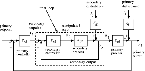
10.3 Cascade-Control Analysis

There are two common ways to represent a cascade-control system in transfer function form: series cascade and parallel cascade. The series cascade representation shown in Figure 10-8 is the most common, so it will be used in the analysis performed in this section. Students interested in analysis using the parallel structure can work Exercise 11.

We use the following algebraic manipulations to understand the effect of the secondary (inner-loop) on the primary (or outer) loop. Notice that the secondary output can be written

Equation 10.1

The secondary closed-loop transfer function can be defined as

Equation 10.2

Further analysis yields

Equation 10.3

After tuning the inner loop, we can use the following transfer function to design the outer-loop controller.

Equation 10.4

and the closed-loop relationship for a primary setpoint change is

Equation 10.5

where it is clear that the secondary closed-loop transfer function affects the primary control loop. Notice that if the secondary control loop is much faster than the primary loop, so that g_c2CL = 1 (on a relative time scale to the primary control loop), then the closed-loop transfer function for the primary loop is