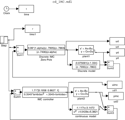
Appendix M16.2: SIMULINK .m and .mdl Files for Example M16.3

Use the following m-file to run simulations based on the cd_IMC.mdl SIMULINK model, and make plots. See Figure M16-5.

% Run continuous and discrete IMC simulations
% For use with the simulink diagram: cd_IMC.mdl
%
% B.W. Bequette
% 14 Sept 00
%
% plant values are (notice the other models are embedded in the
% simulink diagram

  a = [-2.4048 0;0.8333 -2.2381];
  b = [7; -1.117];
  c = [0 1];
  d = 0;
%
% first enter the value of lambda desired in the command window
%
  alpha = exp(-0.1/lambda);
%
  tfinal = 5; % final simulation time
  sim('cd_IMC')
%
  figure(3)
  title('comparison of discrete and continuous IMC')
  subplot(2,1,1),plot(t,yimc,'--',t,yd,t,r,'-.')
  legend('continuous','discrete')
  xlabel('time, min')
  ylabel('y')
  subplot(2,1,2),plot(t,uimc,'--',t,ud)
  legend('continuous','discrete')
  ylabel('u')
  xlabel('time, min')