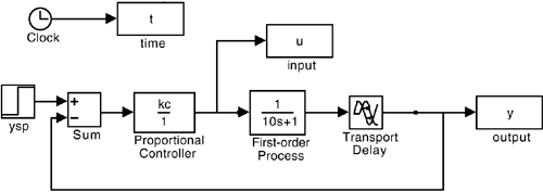
M6.2 Closed-Loop Time-Domain Simulation

Here, we begin by using the SIMULINK diagram shown in Figure M6-1.

Figure M6-1. Simulink diagram. For best results, choose a stiff integrator, such as `ode15s` (stiff/NDF), from the "`parameters`" pull-down menu.

graphics/m06fig01.gif

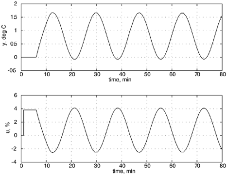
The system is on the verge of instability when k_c = 3.8 %/°C, as shown in Figure M6-2; the ultimate proportional gain is then k_cu = 3.8 %/°C. The period of oscillation (ultimate period, P_u) is approximately 17.2 minutes. Both of these values can be obtained from frequency-response analysis, as shown in Section M6.3. Notice that the manipulated variable action is constant from t = 1 to t = 6 minutes. This is due to the initial "proportional kick." The manipulated input does not change until the process output is observed to change at t = 6 minutes (remember there is a 5-minute time delay). If we used a controller with integral action, the manipulated input would have kept increasing during this interval.

Figure M6-2. Closed-loop response for a setpoint change of 1°C at time = 1 minute, with k_c = 3.8 %/°C. The period of oscillation (P_u, peak-to-peak time) is 17.2 minutes.

graphics/m06fig02.gif

[ Team LiB ]

M6.2 Closed-Loop Time-Domain Simulation

Figure M6-1. Simulink diagram. For best results, choose a stiff integrator, such as ode15s (stiff/NDF), from the "parameters" pull-down menu.

Figure M6-2. Closed-loop response for a setpoint change of 1°C at time = 1 minute, with kc = 3.8 %/°C. The period of oscillation (Pu, peak-to-peak time) is 17.2 minutes.

Figure M6-1. Simulink diagram. For best results, choose a stiff integrator, such as `ode15s` (stiff/NDF), from the "`parameters`" pull-down menu.

Figure M6-2. Closed-loop response for a setpoint change of 1°C at time = 1 minute, with k_c = 3.8 %/°C. The period of oscillation (P_u, peak-to-peak time) is 17.2 minutes.