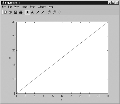
M1.5 Plotting

MATLAB has many nice graphics capabilities. Here, we will illustrate standard two-dimensional plots. First, generate two vectors for plotting

» x = 1:2:11;
» z = 5:5:30;

For a standard solid line plot, simply enter

» plot(x,z)

and Figure M1-2 appears. Axis labels are added by selecting "Insert" and specifying X label or Y label. Alternatively, in the command window you can use the following commands (perform this):

» xlabel('x')
» ylabel('z')

For more plotting options, type

» help plot

If we wish to plot discrete points, using + as a symbol, we can use the following (perform this):

»  plot(x,z,'+')

Notice that a new plot appears in the place of the previous one. You can generate a new figure by entering figure(n), where n is any integer, before entering new plot commands.

Consider now the following equation:

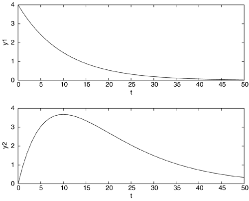
We can plot this for a vector of t values using two simple commands,

» t = 0:1:50;
» y = 4*exp(-0.1*t);

and we can obtain a plot by entering in the command window (perform this)

» figure(2)
» plot(t,y)

Notice that we could shorten the sequence of commands by entering (perform this)

» plot(t,4*exp(-0.1*t))

To perform element-by-element multiplication of two vectors or arrays of the same size, we can use the .* command. We can plot the function y(t) = t·e^–0.1t by using (perform this)

» figure(3)
» y = t.*exp(-0.1*t);
» plot(t,y)
» xlabel('t')
» ylabel('y')

axis('square') will place the plot in a square box, while axis('normal') will change back to a normal aspect ratio.

You can also explicitly set the upper and lower bounds on the plot with

axis([xlow  xhigh  ylow  yhigh])

For this example, we would use

» axis([0  50  0  4]);

Multiple curves can be placed on the same plot in the following fashion (perform this).

» plot(t,4*exp(-0.1*t),t,t.*exp(-0.1*t),'--')

The subplot command can be used to make multiple plots, as illustrated in Figure M1-3.

» subplot(2,1,1), plot(t,4*exp(-0.1*t)), xlabel('t'),ylabel('y1')
» subplot(2,1,2), plot(t,t.*exp(-0.1*t)), xlabel('t'),ylabel('y2')

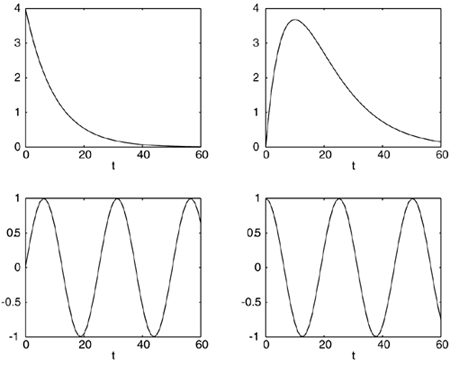
Here, subplot(i,j,k) means that there are i "rows" of figures, j "columns" of figures, and the current plot is the kth figure (counting left to right and top to bottom). The following is an example of a four plot sequence shown in Figure M1-4:

» t = 0:1:60;
» subplot(2,2,1),plot(t,4*exp(-0.1*t)), xlabel('t')
» subplot(2,2,2),plot(t,t.*exp(-0.1*t)), xlabel('t')
» subplot(2,2,3),plot(t,sin(.25*t)), xlabel('t')
» subplot(2,2,4),plot(t,cos(.25*t)), xlabel('t')

To return to single plots, simply enter subplot(1,1,1).